The measurement circuit for obtaining data for curve fitting is the following (LTspice). Input vg1 is stepped over a range to produce the desired range of drain current. The drain current (from VRD), Vd1, and Vd2, are measured, thus Vgs2 and Vds2. The output characteristic is obtained from the circuit by stepping VDD over a range for a given vg1. The device is the Philips HEF4007 CMOS chip. Devices are M1, pins 6, 7, and 8 and M2, 9, 10, and 12. The simulator is the ekv v262 or equivalent.

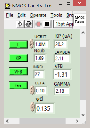
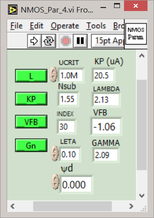
Curve fitting parameter determination (M2) includes GAMMA, which provides NSUB, PHI. Curve fitting (M1) produces KP (UO), LAMBDA, and VFB (VTO). Separate adjustments are made to LETA and UCRIT, for best fits. Measured data (National Instruments DAQ and NI-DAQ) are stored in a Global Variable, as shown.

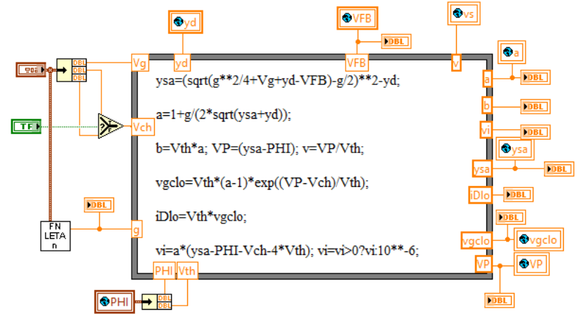
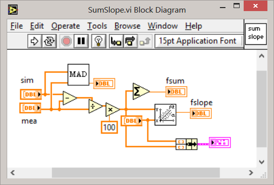
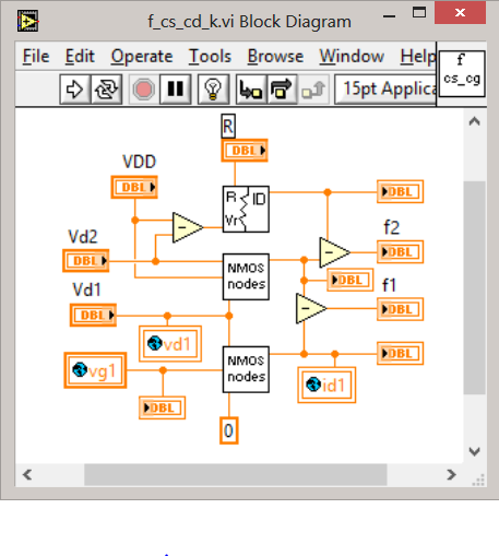
Example application is here, the function which fits the transfer characteristic for KP (sum) and VFB (slope of the difference).

Sum/Slope Computer – The function output (fslope or fsum) is the input to the Newton’s Method Root finder in the curve fitting process. The root-finder loop halts when these values reach a certain specified small value.

Sample Root Finder – KP – VFB and KP are carried as Global Variables to facilitate passing along the updates. Note that in this case the plus and minus increments for the input variable (KP) are 100u with KP about 20 (uA).

Newton’s Method Iteration

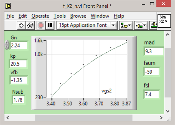
Transfer Function Fit – KP and VFB – MAD is mean absolute point difference, percent.
M2 Transfer Characteristic – Sample GAMMA, NSUB.

With Curve Fit.

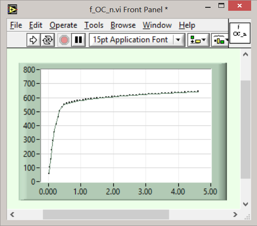
Output Characteristic Curve Fit
Simulator uses ekv channel-length modulation function and LETA function.


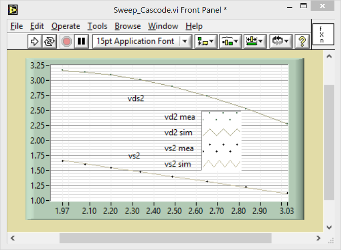
Simulated and Measured comparison.

Cascode Root Finder Functions (vd1 and vd2 iterations).